Fitting Time Series Models to Nonstationary Processes
Basic Structural Model & Dynamic Linear Model using R
State Space Model and Kalman Filter for Time-Series Prediction
Time-series forecasting using financial data
![]()
https://sarit-maitra.medium.com/membership
T ime series consist of four major components: Seasonal variations (SV), Trend variations (TV), Cyclical variations (CV), and Random variations (RV). Here, we will perform predictive analytics using state space model on uni-variate time series data. This model has continuous hidden and observed state.
State space model
Let us use historical data of Schlumberger Limited (SLB) from 1986 onwards.
Line plot
          df1 = ts(df1$Open, start= c(1986,1), end = c(2019,12), frequency = 12)
xyplot(df1, ylab = "Price (US $)", main = "Time series plot for Schlumberger price")
Here, data is on monthly frequency (12 months) for the ease of computation.
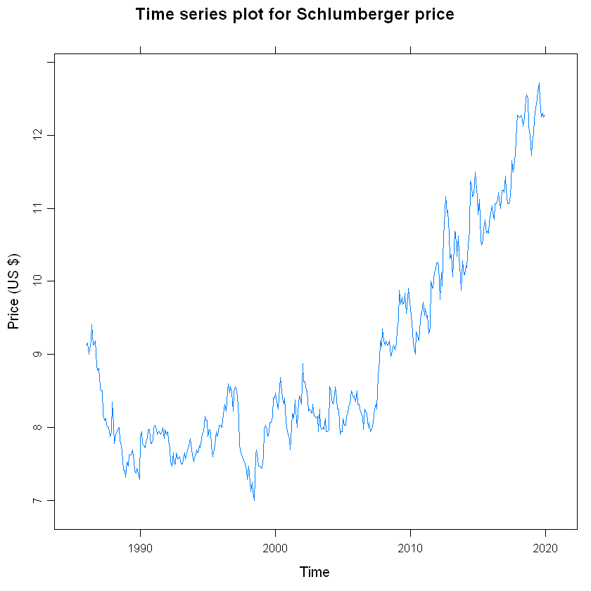
The line plot shows fluctuating price all throughout with high volatility.
Density & Q-Q plot
The distribution plot comprising density and normal QQ plot below clearly shows that data distribution is not normal.
          par(mfrow=c(2,1)) # set up the graphics
hist(df1, prob=TRUE, 12) # histogram
lines(density(df1)) # density for details
qqnorm(df1) # normal Q-Q plot
qqline(df1) 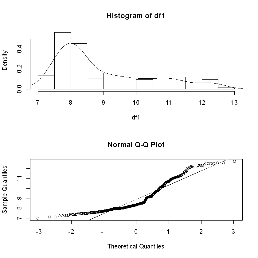
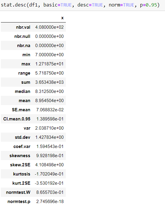
Descriptive Statistic
Stationarity test
Le t us perform stationarity test (ADF, Phillips-Perron & KPSS) on original data.
stationary.test(df1, method = "adf")
stationary.test(df1, method = "pp") # same as pp.test(x)
stationary.test(df1, method = "kpss") Augmented Dickey-Fuller Test
alternative: stationaryType 1: no drift no trend
lag ADF p.value
[1,] 0 0.843 0.887
[2,] 1 0.886 0.899
[3,] 2 0.937 0.906
[4,] 3 0.924 0.904
[5,] 4 0.864 0.893
[6,] 5 1.024 0.917
Type 2: with drift no trend
lag ADF p.value
[1,] 0 -0.1706 0.936
[2,] 1 -0.0728 0.950
[3,] 2 -0.0496 0.952
[4,] 3 -0.0435 0.952
[5,] 4 -0.0883 0.947
[6,] 5 0.3066 0.978
Type 3: with drift and trend
lag ADF p.value
[1,] 0 -2.84 0.224
[2,] 1 -2.83 0.228
[3,] 2 -2.72 0.272
[4,] 3 -2.79 0.242
[5,] 4 -2.96 0.172
[6,] 5 -2.96 0.173
----
Note: in fact, p.value = 0.01 means p.value <= 0.01
Phillips-Perron Unit Root Test
alternative: stationaryType 1: no drift no trend
lag Z_rho p.value
5 0.343 0.768
-----
Type 2: with drift no trend
lag Z_rho p.value
5 -0.0692 0.953
-----
Type 3: with drift and trend
lag Z_rho p.value
5 -11.6 0.386
---------------
Note: p-value = 0.01 means p.value <= 0.01
KPSS Unit Root Test
alternative: nonstationaryType 1: no drift no trend
lag stat p.value
4 0.261 0.1
-----
Type 2: with drift no trend
lag stat p.value
4 0.367 0.0914
-----
Type 1: with drift and trend
lag stat p.value
4 0.123 0.0924
-----------
Note: p.value = 0.01 means p.value <= 0.01
: p.value = 0.10 means p.value >= 0.10
Data normalization
I have normalized the dataset using mean and std. dev.
Auto-correlation Function (ACF)
Identify if correlation at different time lags goes to 0
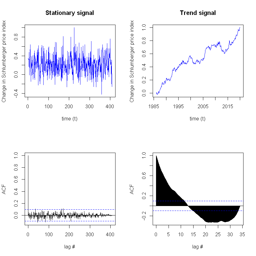
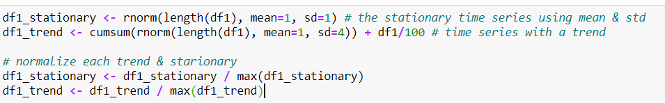
The stationary = Gaussian noise and one with a trend = cumulative sum of Gaussian noise.
Here, we will check each for characteristics of stationarity by looking at the auto-correlation functions of each signal. We would expect the ACF to go to 0 for each time lag (τ) for a stationary signal, because we expect no dependence with time.
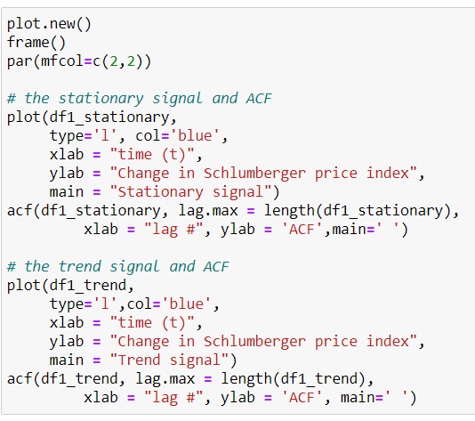
We see here that, the stationary signal has very few lags exceeding the CI of the ACF . The trend resulted in almost all lags exceeding the confidence interval. It can be concluded that the ACF signal is stationary. But, the trend signal is not stationary . The stationary series has a better variance around the mean level, and the peaks are evidence of the interventions in the original series.
We will further decompose the time series which involves a combination of level, trend, seasonality, and noise components. Decomposition helps to provide a better understanding of problems during analysis and forecasting.
Decomposing Time Series
We may apply differencing the data or log transform the data to eliminate trend and seasonality. Such process may not be a shortcoming if we are only concerned with forecasting. However, in many contexts of statistics and econometric application, knowledge of this components has underlying importance. Estimates of trend & seasonal can be recovered from differenced series by maximizing the residual mean square but this is not as appealing as modeling the components directly. We have to remember that, real series are never stationary.
Here, we will use simple moving average smoothing method of the time series to estimate the trend component.
          df1SMA8 <- SMA(df1, n=8) # smoothing with moving average 8
plot.ts(df1SMA8) 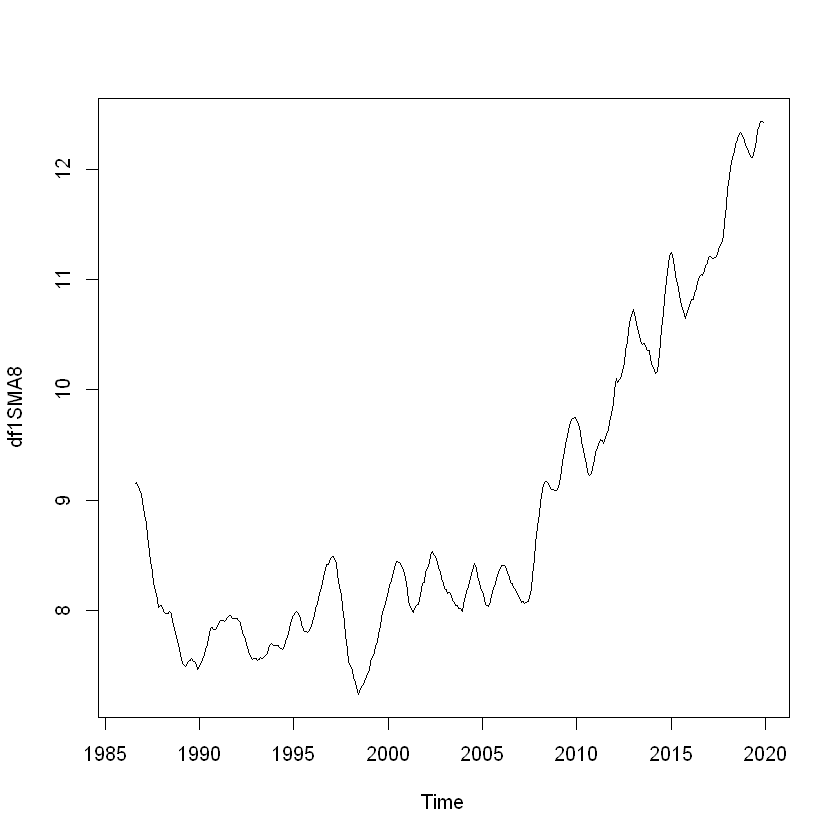
          df1Comp <- decompose(df1SMA8) # decomposing
plot(df1Comp, yax.flip=TRUE) 
The plot shows the original time series (top), the estimated trend component (second from top), the estimated seasonal component (third from top), and the estimated irregular component (bottom).
We see that the estimated trend component shows a small decrease from about 9 in 1997 to about 7 in 1999, followed by a steady increase from then on to about 12 in 2019.
Seasonally Adjusting
          df1.Comp.seasonal <- sapply(df1Comp$seasonal, nchar)
df1SeasonAdj <- df1 — df1.Comp.seasonal
plot.ts(df1SeasonAdj) 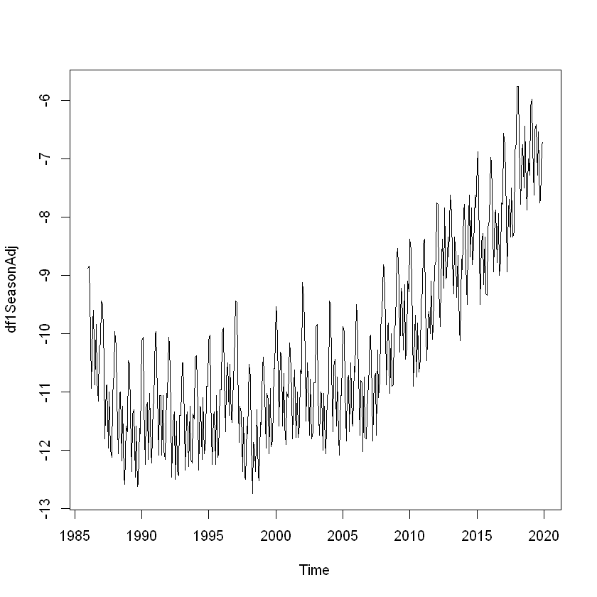
We will also explore Kalman filter for series filtering & smoothening purpose prior to prediction.
Structural model
Structural time series models are (linear Gaussian) state-space models for (uni-variate) time series. When considering state space architecture, normally we are interested in considering three primary areas:
- Prediction which is forecasting subsequent values of the state
- Filtering which is estimating the current values of the state from past and current observations
- Smoothing which is estimating the past values of the state given the observations
We will use Kalman Filter to carry out the various types of inference.
Filtering helps us to update our knowledge of the system as each observation comes in. Smoothing helps us to base our estimates of quantities of interest on the entire sample.
Basic structural model (BSM)
Structural mode has the advantage of being of simple usage and quite reliable. It gives the main tools for fitting a structural model for a time series by maximum likelihood.
Structural time series state-space model based on a decomposition of the series into a number of components. They are specified by a set of error variances, some of which may be zero. We will use a basic structural model to fit the stochastic level model to forecast. The two main components which make up state space models are (1) an observed data and (2) the unobserved states.
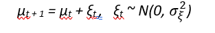
The simplest model is the local level model has an underlying level µt which evolves by:
We need to see the observations, since the states are hidden to us by system noise. The observations are a linear combination of the current state and some additional random variation known as measurement noise. The observations are:
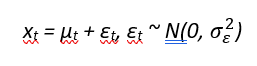
It is in fact an ARIMA(0,1,1) model, but with restrictions on the parameter set. This is stochastically varying level (random walk) observed with noise.
The local linear trend model has the same measurement equation, but with a time-varying slope in the dynamics for µt, given by
with three variance parameters. Here εt , ξt and ζt are independent Gaussian white noise processes. The basic structural model, is a local trend model with an additional seasonal component. Thus the measurement equation is:
where γt is a seasonal component with dynamics
Train/Test split
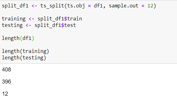
Model fitting and prediction
It's best practice to check the convergence of the structural procedure. As with any structural process we need to have appropriate initial starting points to ensure the algorithm will converge to the right maximum.
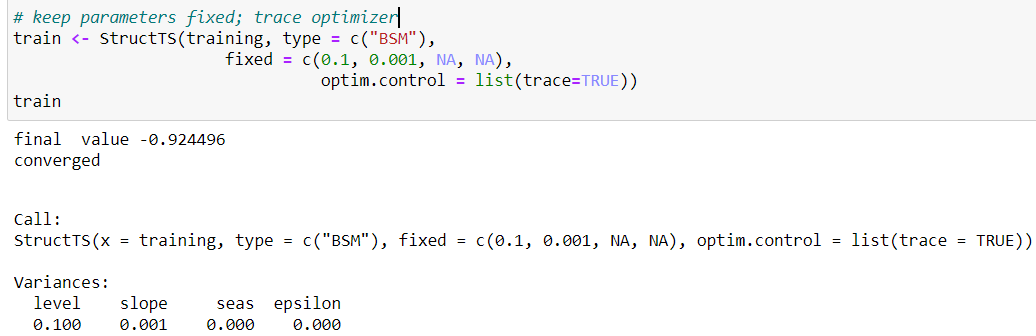
autoplot(training, series="Training data") + autolayer(fitted(train, h=12), series="12-step fitted values") 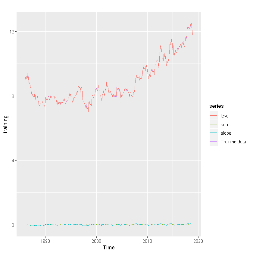
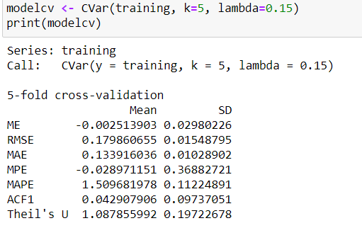
Cross validation
Cross validation is an important step of time series analysis.
- Fit model to data y1, . . . , yt
- Generate 1-step ahead forecast ˆyt+1
- Compute forecast error e ∗ t+1 = yt+1 − yˆt+1
- Repeat steps 1–3 for t = m, . . . , n − 1 where m is minimum number of observations to fit model
- Compute forecast MSE from e ∗ m+1, . . . , e ∗
The p-value of Ljung-Box test of residuals is 0.2131015 > significant level(0.05); therefore, it is not advisable to use the result of the cross-validation as the model is clearly under-fitting the data.
Basic diagnostics
The first diagnostic that we do with any statistical analysis is check that our residuals correspond to our assumed error structure. We have two types of errors in a uni-variate state-space model: process errors, the wt, and observation errors, the vt. They should not have a temporal trend.
model.residuals
vt are the difference between the data and the predicted data at time t: vt = yt − Zxt − a
In a state-space model, xt is stochastic and the model residuals are a random variable. yt is also stochastic, though often observed unlike xt. The model residual random variable is: Vt = Yt − ZXt − a
The unconditional mean and variance of Vt is 0 and R
checkresiduals(train) 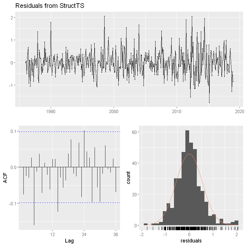
Kalman filter
Kalman filter algorithm uses a series of measurements observed over time, containing noise and other inaccuracies, and produces estimates of unknown variables. This estimate tend to be more accurate than those based on a single measurement alone. Using a Kalman filter does not assume that the errors are Gaussian; however, the filter yields the exact conditional probability estimate in the special case that all errors are Gaussian.
Kalman filter is a means to find the estimates of the process. Filtering comes from its primitive use of reducing or "filtering out" unwanted variables which in our case is the estimation error.
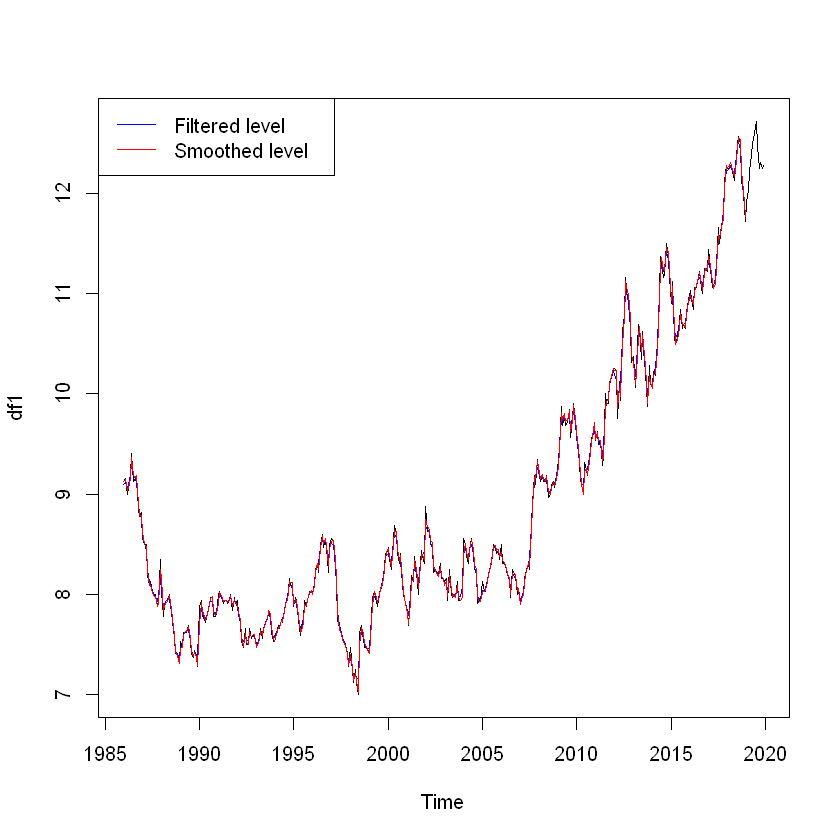
          sm <- tsSmooth(train)
plot(df1)
lines(sm[,1],col='blue')
lines(fitted(train)[,1],col='red')          # Seasonally adjusted data
training.sa <- df1 — sm[, 1]
lines(training.sa, col='black')
legend("topleft",col=c('blue', 'red', 'black'), lty=1,
            legend=c("Filtered level", "Smoothed level")
          x <- training
miss <- sample(1:length(x), 12)
x[miss] <- NA
estim <- sm[,1] + sm[, 2]
plot(x, ylim=range(df1))
points(time(x)[miss], estim[miss], col = 'red', pch = 1)
points(time(x)[miss], df1[miss], col = 'blue', pch = 1)
legend("topleft", pch = 1, col = c(2,1), legend = c("Estimate", "Actual")) 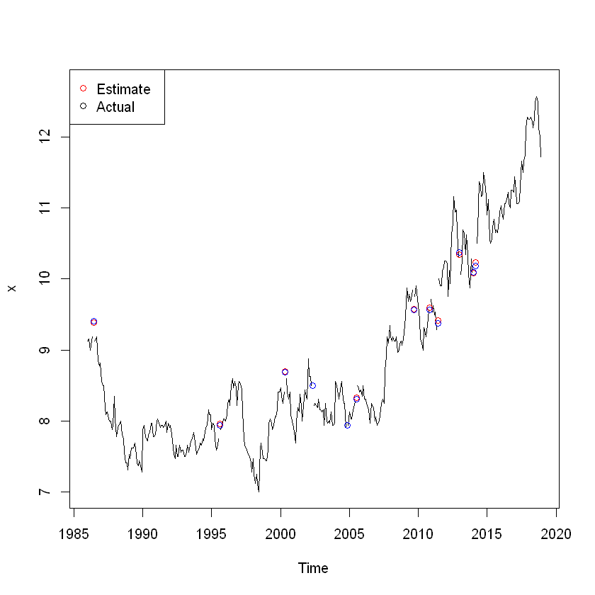
          plot(sm, main = "")
mtext(text = "decomposition of the basic structural", side = 3, adj = 0, line = 1) 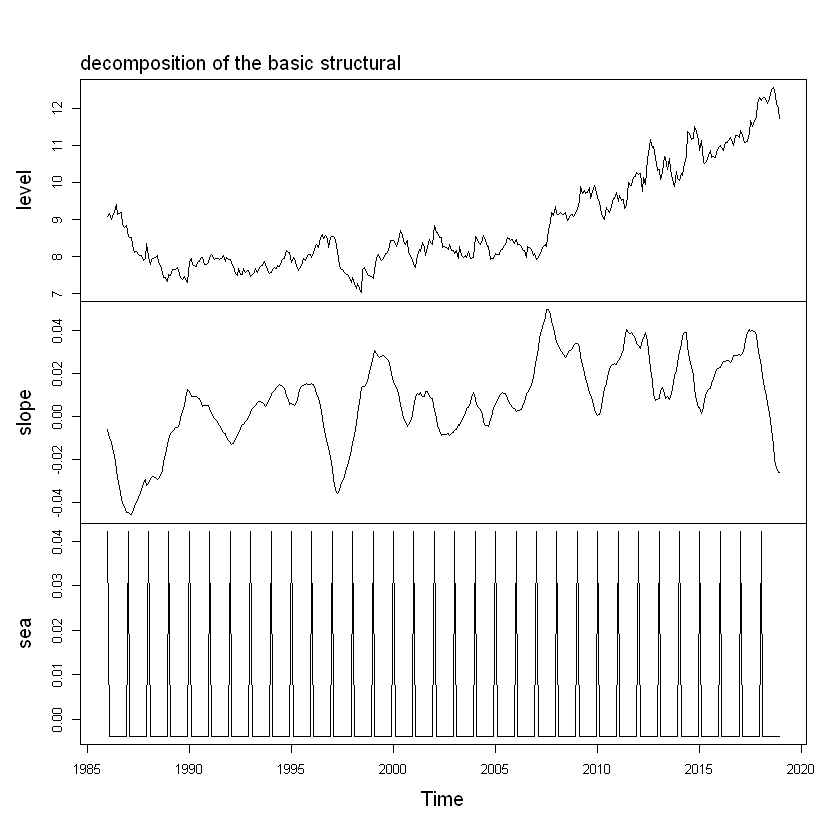
Prediction
          sm %>%
            forecast(h=12) %>%
            autoplot() + autolayer(testing)
Below plot shows the foretasted Schlumberger data together with 50% and 90% probability intervals.
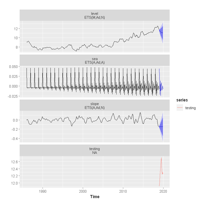
As we can see that, BSM model is been able to pick up the seasonal component quite well . One can experiment here with SMA based decomposition ( as shown earlier) and compare the forecast accuracy.
Dynamic Linear Model (dlm) with Kalman filter
dlm models are a special case of state space models where the errors of the state and observed components are normally distributed. Here, Kalman filter will be used to:
- filtered values of state vectors.
- smoothed values of state vectors and finally,
- forecast provides means and variances of future observations and states.
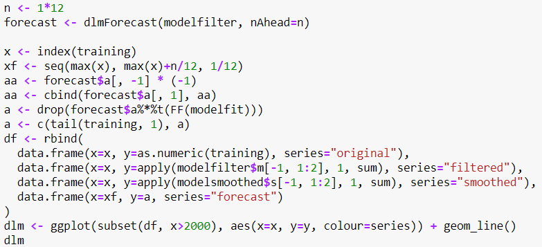
We have to define the parameters before fitting a dlm model. The parameters are V, W (covariance matrices of the measurement and state equations, respectively), FF and GG (measurement equation matrix and transition matrix respectively), and m0, C0 (prior mean and covariance matrix of the state vector).
However, here, we start the dlm model by writing a small function as below:
I have considered a local level model with dlm A polynomial DLM (a local linear trend is a polynomial DLM of order 2) and seasonal component 12. It's good practice rather part of best practice to check the convergence of the MLE procedure.
Kalman filter and smoother have been applied as well.
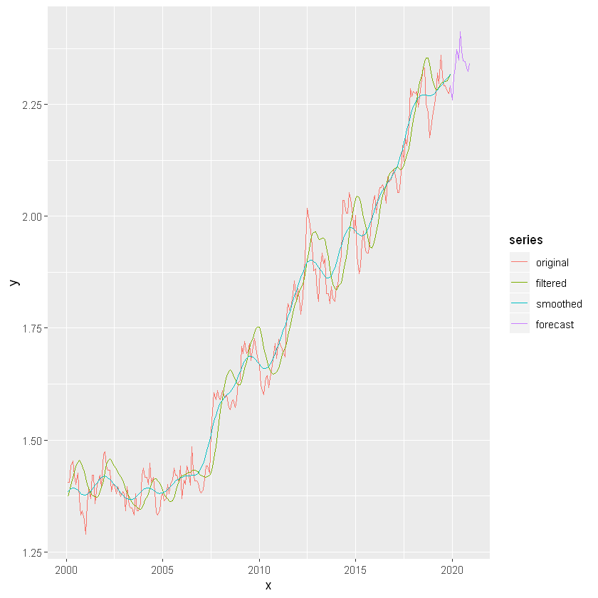
We can see that, dlm model's prediction accuracy fairly well. Filter and smooth lines are almost moving together in the series and do not differ much from each other. The seasonal components are ignored here. The lines of forecast series and the original series are quite close.
A good example of state-space models with time series analysis can be found here .
Summary
State space models come in lots of flavors and a flexible way of handling lots of time series models and provide a framework for handling missing values, likelihood estimation, smoothing, forecasting, etc. Both uni-variate and multi-variate data can be used to fit state space model. We have shown a basic level model in this exercise.
I can be reached here .
Reference:
- Durbin, J., & Koopman, S. J. (2012). Time series analysis by state space methods. Oxford university press.
- Giovanni Petris & Sonia Petrone (2011), State Space Models in R, Journal of Statistical Software
- G Petris, S Petrone, and P Campagnoli (2009). Dynamic Linear Models with R. Springer
- Hyndman, R. J., & Athanasopoulos, G. (2018). Forecasting: principles and practice. OTexts.
Fitting Time Series Models to Nonstationary Processes
Source: https://towardsdatascience.com/state-space-model-and-kalman-filter-for-time-series-prediction-basic-structural-dynamic-linear-2421d7b49fa6